Overview
When data arrives continuously — from sensors, logs, or streaming pipelines — you need incremental smoothing that doesn’t require reprocessing the entire dataset.
Online Mode: Point-by-Point
For true real-time applications where each point must be processed immediately.
window_capacity = 25 limits the internal buffer to the
25 most recent observations; each add_point call costs
O(window) rather than growing with total history.
min_points = 5 suppresses output until the window holds
enough points for a stable fit — calls made before that threshold return
NULL. update_mode = "incremental" re-fits only
the most recent point rather than the full window, halving typical
latency at a modest accuracy cost.
Sensor Data Example
library(rfastloess)

set.seed(42)
times        <- 1:100
temperatures <- 20 + 5 * sin(times / 10) + rnorm(100)

model <- OnlineLoess(
    fraction = 0.3,
    window_capacity = 25,
    min_points = 5,
    update_mode = "incremental"
)
for (i in seq_along(times)) {
    result <- add_point(model, times[i], temperatures[i])
    if (!is.null(result))
        cat(sprintf("Time %d: %.2f\n", times[i], result$y))
    if (i >= 10) break  # print only the first few outputs
}
#> Time 5: 22.80
#> Time 6: 22.72
#> Time 7: 24.73
#> Time 8: 23.49
#> Time 9: 25.94
#> Time 10: 24.14
Accumulating Results
library(rfastloess)
set.seed(42)
n      <- 200
times  <- seq_len(n)
signal <- 10 + 2 * sin(times / 20) + rnorm(n, sd = 1)

model <- OnlineLoess(
    fraction        = 0.3,
    window_capacity = 30,
    min_points      = 5
)

smoothed_x <- numeric(n)
smoothed_y <- numeric(n)
n_out <- 0L

for (i in seq_len(n)) {
    result <- add_point(model, times[i], signal[i])
    if (!is.null(result)) {
        n_out <- n_out + 1L
        smoothed_x[n_out] <- times[i]
        smoothed_y[n_out] <- result$y
    }
}

smoothed_x <- smoothed_x[seq_len(n_out)]
smoothed_y <- smoothed_y[seq_len(n_out)]

plot(times, signal, pch = 16, cex = 0.4, col = "gray",
    xlab = "Time", ylab = "Value",
    main = "Online LOESS — Accumulated Output")
lines(smoothed_x, smoothed_y, col = "blue", lwd = 2)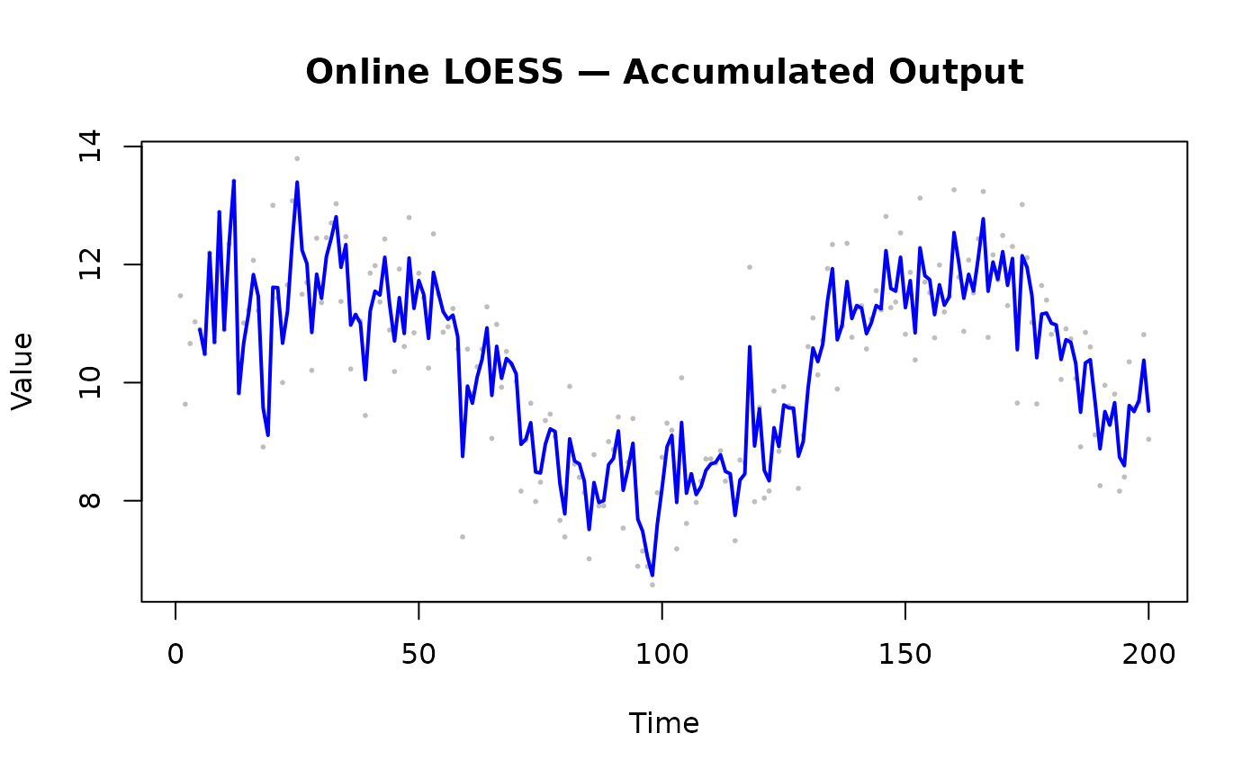
Streaming Mode: Chunk Processing
For large datasets that arrive in batches or files.
chunk_size controls how many data points are processed
in one pass; matching it to your file-read buffer or message-batch size
avoids unnecessary copying. overlap retains that many
points from the previous chunk as context so the neighbourhood at chunk
boundaries is not artificially truncated.
merge_strategy = "weighted_average" blends the overlapping
region smoothly; use "take_last" if chunk boundaries are
guaranteed to be well separated and no blending is needed.
Always call finalize(): The streaming adapter buffers overlap data. Call
finalize(model)after the last chunk to retrieve the buffered tail.
Log File Processing
library(rfastloess)
set.seed(42)

total_points <- 100000
x <- 0:(total_points - 1)
y <- sin(x / 1000) + rnorm(total_points, sd = 0.1)

model <- StreamingLoess(
    fraction       = 0.05,
    chunk_size     = 10000,
    overlap        = 1000,
    merge_strategy = "weighted_average"
)
process_chunk(model, x, y)
#> <LoessResult>
#>   Points:            99000
#>   Fraction Used:     0.05
#>   Iterations Used:   3
result <- finalize(model)
cat("Processed", length(result$y), "points\n")
#> Processed 1000 points
Real-Time Dashboard Example
The dashboard pattern uses a plain LOESS fit on a manually managed
sliding window rather than OnlineLoess. This is the
simplest approach when your UI framework already owns the data buffer
and you only need the most recent smoothed value per frame. The
trade-off is a full O(window^2) refit on every tick; for high-frequency
streams prefer OnlineLoess with
update_mode = "incremental" to bound per-frame cost.
library(rfastloess)
set.seed(42)

window_capacity <- 50
data_x <- numeric(0)
data_y <- numeric(0)

for (i in 0:199) {
    xi <- i
    yi <- 25.0 + 10 * sin(i / 20) + rnorm(1, sd = 2)
    data_x <- c(data_x, xi)
    data_y <- c(data_y, yi)

    if (length(data_x) > window_capacity) {
        data_x <- tail(data_x, window_capacity)
        data_y <- tail(data_y, window_capacity)
    }

    if (length(data_x) >= 5) {
        model <- Loess(fraction = 0.4)
        result <- fit(model, data_x, data_y)
        current_smoothed <- tail(result$y, 1)
    }
}
Choosing Parameters
Performance Considerations
| Mode | Memory | Latency | Use Case |
|---|---|---|---|
| Online | Fixed (window) | ~1ms/point | Sensors, dashboards |
| Streaming | ~chunk_size | ~100ms/chunk | Large files, ETL |
| Batch | Full dataset | N/A | Analysis, reports |
See Also
-
vignette("adapter-choice", package = "rfastloess")— Detailed mode comparison -
vignette("merge", package = "rfastloess")— Chunk reconciliation in depth -
vignette("scaling", package = "rfastloess")— Robustness scale estimation -
vignette("use-case-time-series", package = "rfastloess")— General time series analysis
sessionInfo()
#> R version 4.6.1 (2026-06-24)
#> Platform: x86_64-pc-linux-gnu
#> Running under: Ubuntu 24.04.5 LTS
#>
#> Matrix products: default
#> BLAS:   /usr/lib/x86_64-linux-gnu/openblas-pthread/libblas.so.3
#> LAPACK: /usr/lib/x86_64-linux-gnu/openblas-pthread/libopenblasp-r0.3.26.so;  LAPACK version 3.12.0
#>
#> locale:
#>  [1] LC_CTYPE=C.UTF-8       LC_NUMERIC=C           LC_TIME=C.UTF-8
#>  [4] LC_COLLATE=C.UTF-8     LC_MONETARY=C.UTF-8    LC_MESSAGES=C.UTF-8
#>  [7] LC_PAPER=C.UTF-8       LC_NAME=C              LC_ADDRESS=C
#> [10] LC_TELEPHONE=C         LC_MEASUREMENT=C.UTF-8 LC_IDENTIFICATION=C
#>
#> time zone: UTC
#> tzcode source: system (glibc)
#>
#> attached base packages:
#> [1] stats     graphics  grDevices utils     datasets  methods   base
#>
#> other attached packages:
#> [1] rfastloess_3.0.0
#>
#> loaded via a namespace (and not attached):
#>  [1] digest_0.6.39     desc_1.4.3        R6_2.6.1          fastmap_1.2.0
#>  [5] xfun_0.62         cachem_1.1.0      knitr_1.52        htmltools_0.5.9
#>  [9] rmarkdown_2.32    lifecycle_1.0.5   cli_3.6.6         sass_0.4.10
#> [13] pkgdown_2.2.1     textshaping_1.0.5 jquerylib_0.1.4   systemfonts_1.3.2
#> [17] compiler_4.6.1    tools_4.6.1       ragg_1.5.2        bslib_0.12.0
#> [21] evaluate_1.0.5    yaml_2.3.12       otel_0.2.0        jsonlite_2.0.0
#> [25] rlang_1.3.0       fs_2.1.0          htmlwidgets_1.6.4