Basic Trend Extraction
fraction = 0.1 sizes the neighbourhood as 10% of the
data at each evaluation point — narrow enough to follow a slowly varying
trend without smearing periodic variation. Three robustness
iterations down-weight noise spikes so they cannot bias the
fitted curve; this is especially important when the signal-to-noise
ratio is low or when occasional outliers are expected.
library(rfastloess)

set.seed(42)
t <- seq(0, 100, length.out = 500)
trend <- 10 + 0.5 * t + 3 * sin(t / 10)
noise <- rnorm(500, sd = 3)
y <- trend + noise

model <- Loess(fraction = 0.1, iterations = 3)
result <- fit(model, t, y)

plot(t, y, col = "gray", pch = ".",
    xlab = "Time", ylab = "Value", main = "Trend Extraction")
lines(result$x, result$y, col = "blue", lwd = 2)
legend("topleft", c("Observed", "Trend (LOESS)"),
        pch = c(1, NA), lty = c(NA, 1), col = c("gray", "blue"))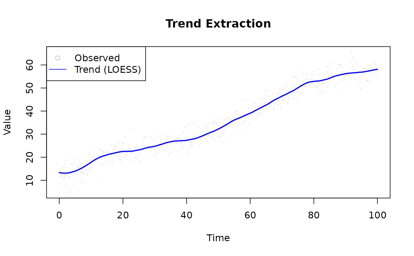
Seasonal Decomposition
Setting outputs = "residuals" stores
observed − smoothed alongside the smooth. A slightly wider
fraction = 0.4 produces a smoother baseline trend, so
short-duration oscillations end up in the residuals rather than being
absorbed into the trend component. The residual series is then ready for
spectral analysis, seasonality detection, or change-point methods.
library(rfastloess)
set.seed(42)

t        <- 1:120
trend    <- 100 + 0.5 * t
seasonal <- 15 * sin(2 * pi * t / 12)
noise    <- rnorm(120, sd = 5)
y        <- trend + seasonal + noise

model    <- Loess(fraction = 0.4, iterations = 2, outputs = "residuals")
result   <- fit(model, t, y)
residual <- result$residuals

par(mfrow = c(2, 1), mar = c(4, 4, 2, 0.5))
plot(t, y, type = "l", col = "gray",
    main = "Original + LOESS Trend", xlab = "Month", ylab = "Value")
lines(result$x, result$y, col = "blue", lwd = 2)

plot(t, residual, type = "l", col = "darkgreen",
    main = "Detrended Residual (Seasonal Component)",
    xlab = "Month", ylab = "Residual")
abline(h = 0, lty = 2, col = "red")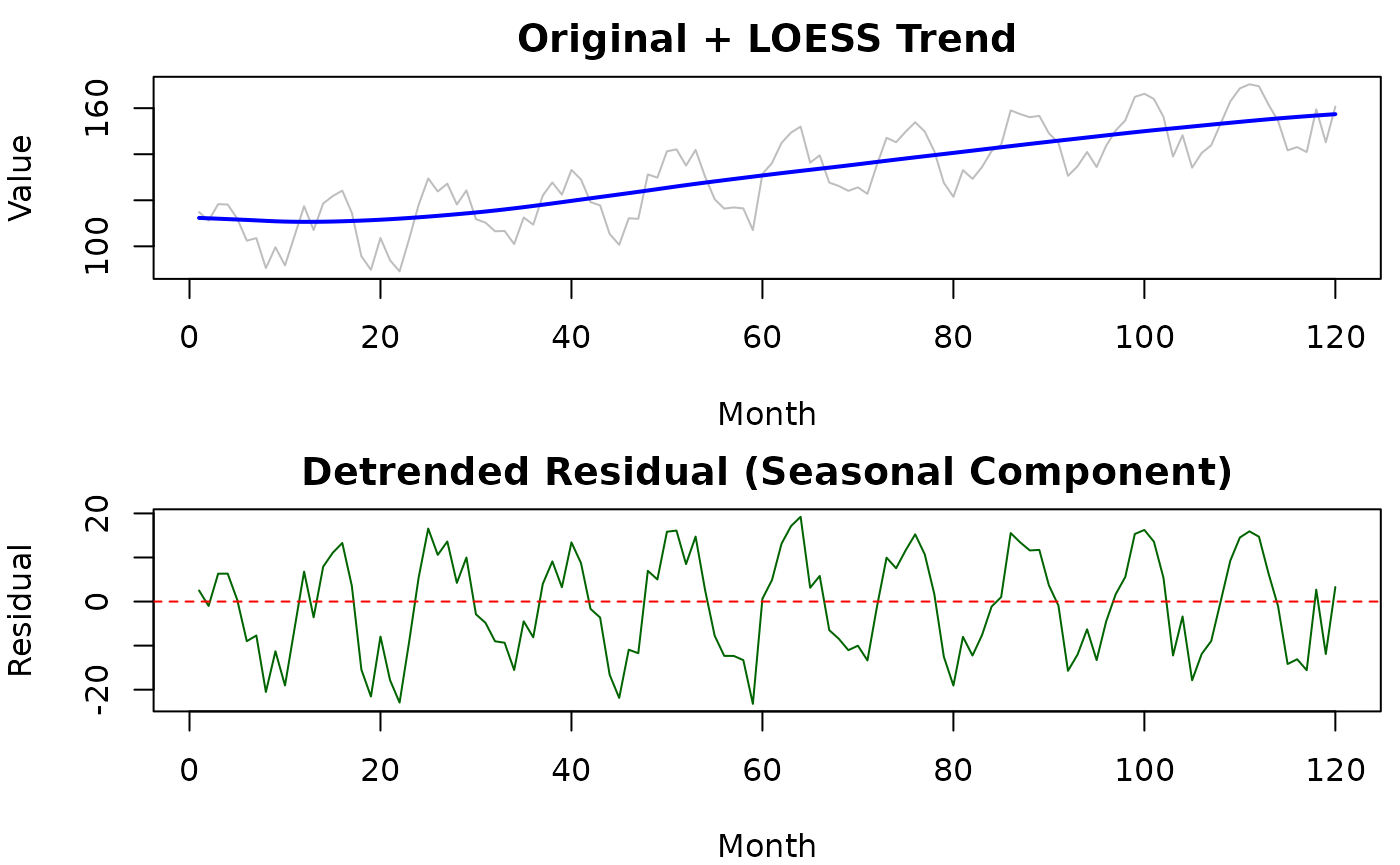
Irregular Time Grids
library(rfastloess)
set.seed(42)

t_irregular <- c(sort(runif(200, 0, 50)), sort(runif(50, 50, 100)))
y_irregular <- sin(t_irregular / 10) + rnorm(length(t_irregular), sd = 0.5)

model  <- Loess(fraction = 0.2, iterations = 2)
result <- fit(model, t_irregular, y_irregular)

plot(t_irregular, y_irregular, pch = 16, cex = 0.4, col = "gray",
    xlab = "Time", ylab = "Value", main = "Irregularly Sampled Time Series")
lines(result$x, result$y, col = "blue", lwd = 2)
Forecasting with Prediction Intervals
Prediction intervals widen the uncertainty band to include both the
uncertainty in the fitted curve (confidence interval) and the expected
scatter of new observations around it. fraction = 0.2
offers a balance between local detail and stable interval width — too
small a fraction produces jagged interval edges; too large a fraction
underestimates local variance near turning points.
library(rfastloess)
set.seed(42)
t <- seq(0, 100, length.out = 500)
y <- 10 + 0.3 * t + sin(t / 5) + rnorm(500, sd = 2)

model <- Loess(
    fraction = 0.2,
    iterations = 3,
    intervals = intervals_opts(confidence = 0.95, prediction = 0.95)
)
result <- fit(model, t, y)

plot(t, y, pch = ".", col = "gray",
    xlab = "Time", ylab = "Value",
    main = "Trend with 95% Prediction Interval")
polygon(c(result$x, rev(result$x)),
        c(result$prediction_upper, rev(result$prediction_lower)),
        col = rgb(0, 0, 1, 0.15), border = NA)
lines(result$x, result$y, col = "blue", lwd = 2)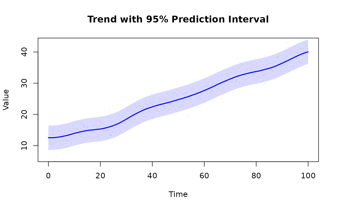
Handling Missing Data
LOESS naturally handles irregular time sampling:
library(rfastloess)
set.seed(42)

t_irregular <- sort(runif(200, 0, 100))
y_irregular <- 10 + t_irregular * 0.3 + rnorm(200, sd = 2)

model <- Loess(fraction = 0.2)
result <- fit(model, t_irregular, y_irregular)
cat("Smoothed y[0]:", result$y[1], "\n")
#> Smoothed y[0]: 12.10549
Multi-Scale Analysis
Use different fractions to extract features at different scales:
library(rfastloess)
set.seed(42)
t <- seq(0, 100, length.out = 500)
trend_true <- 10 + 0.5 * t + 3 * sin(t / 10)
y <- trend_true + rnorm(length(t), sd = 3)

fractions <- c(0.05, 0.2, 0.5)

plot(t, y, col = "gray", pch = ".",
    xlab = "Time", ylab = "Value", main = "Multi-Scale LOESS")

for (f in fractions) {
    model <- Loess(fraction = f)
    result <- fit(model, t, y)
    lines(result$x, result$y, lwd = 2)
}
legend("topleft", paste0("fraction=", fractions), lty = 1)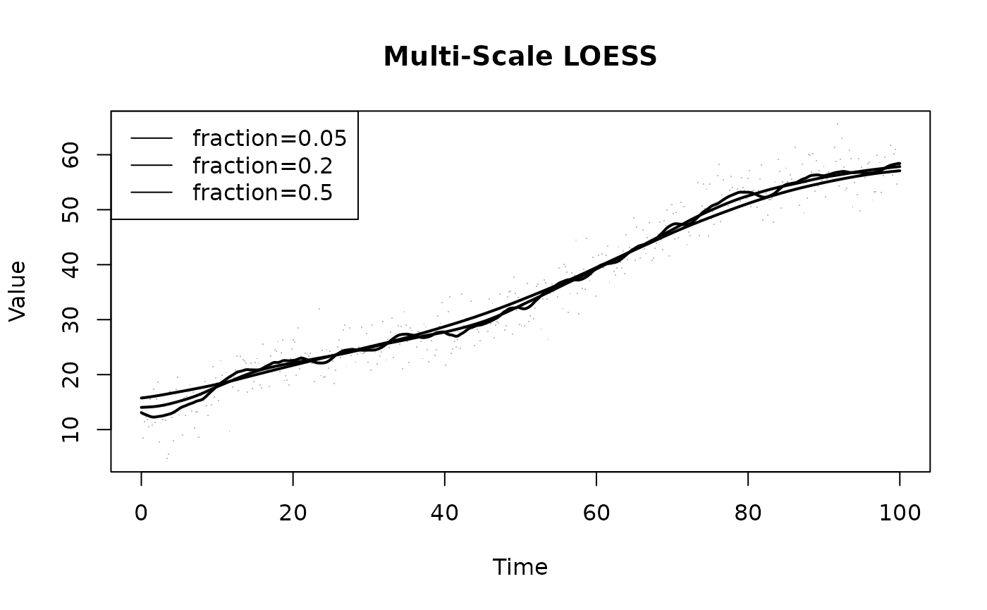
Gene Expression Time Course
Biological application:
library(rfastloess)
set.seed(42)

hours <- seq(0, 24, by = 0.5)
expression <- 100 * (1 + 0.5 * sin(hours * pi / 12)) +
    rnorm(length(hours), sd = 10)

model <- Loess(
    fraction = 0.3,
    iterations = 3,
    outputs = "diagnostics",
    intervals = intervals_opts(confidence = 0.95)
)
result <- fit(model, hours, expression)

cat("R2:", result$diagnostics$r_squared, "\n")
#> R2: 0.9096872
Choosing Fraction for Time Series
| Data Type | Recommended Fraction | Rationale |
|---|---|---|
| Daily data (years) | 0.3–0.5 | Capture annual trends |
| Hourly data (days) | 0.1–0.2 | Capture daily patterns |
| Sensor data (minutes) | 0.05–0.1 | Preserve short-term features |
| Noisy data | Higher | Reduce noise impact |
| Clean data | Lower | Preserve detail |
See Also
-
vignette("use-case-real-time", package = "rfastloess")— For streaming time series -
vignette("cross-validation", package = "rfastloess")— Optimal fraction selection -
vignette("degree", package = "rfastloess")— Degree 2 for curved trends -
vignette("boundary", package = "rfastloess")— Edge bias in trend extraction -
?Loess— Full parameter reference
sessionInfo()
#> R version 4.6.1 (2026-06-24)
#> Platform: x86_64-pc-linux-gnu
#> Running under: Ubuntu 24.04.5 LTS
#>
#> Matrix products: default
#> BLAS:   /usr/lib/x86_64-linux-gnu/openblas-pthread/libblas.so.3
#> LAPACK: /usr/lib/x86_64-linux-gnu/openblas-pthread/libopenblasp-r0.3.26.so;  LAPACK version 3.12.0
#>
#> locale:
#>  [1] LC_CTYPE=C.UTF-8       LC_NUMERIC=C           LC_TIME=C.UTF-8
#>  [4] LC_COLLATE=C.UTF-8     LC_MONETARY=C.UTF-8    LC_MESSAGES=C.UTF-8
#>  [7] LC_PAPER=C.UTF-8       LC_NAME=C              LC_ADDRESS=C
#> [10] LC_TELEPHONE=C         LC_MEASUREMENT=C.UTF-8 LC_IDENTIFICATION=C
#>
#> time zone: UTC
#> tzcode source: system (glibc)
#>
#> attached base packages:
#> [1] stats     graphics  grDevices utils     datasets  methods   base
#>
#> other attached packages:
#> [1] rfastloess_3.0.0
#>
#> loaded via a namespace (and not attached):
#>  [1] digest_0.6.39     desc_1.4.3        R6_2.6.1          fastmap_1.2.0
#>  [5] xfun_0.62         cachem_1.1.0      knitr_1.52        htmltools_0.5.9
#>  [9] rmarkdown_2.32    lifecycle_1.0.5   cli_3.6.6         sass_0.4.10
#> [13] pkgdown_2.2.1     textshaping_1.0.5 jquerylib_0.1.4   systemfonts_1.3.2
#> [17] compiler_4.6.1    tools_4.6.1       ragg_1.5.2        bslib_0.12.0
#> [21] evaluate_1.0.5    yaml_2.3.12       otel_0.2.0        jsonlite_2.0.0
#> [25] rlang_1.3.0       fs_2.1.0          htmlwidgets_1.6.4