Use Case: Genomic Data Smoothing

LOWESS for methylation profiles, ChIP-seq signals, and other genomic data.

Overview

Genomic data often contains noise from sequencing depth variation, PCR artifacts, or biological heterogeneity. LOWESS smoothing helps reveal underlying patterns.

---

Methylation Profile Smoothing

The Challenge

DNA methylation data (from bisulfite sequencing or arrays) shows position-dependent patterns that can be obscured by measurement noise.

Solution

A small fraction = 0.1 lets LOWESS follow fine-scale spatial structure without smearing the transitions between methylated and unmethylated regions. intervals = intervals_opts(confidence = 0.95) produces uncertainty bands that naturally widen at positions with sparser CpG coverage, making low-confidence segments immediately apparent in the plot.

library(rfastlowess)

positions <- seq(0, 99000, by = 1000)
observed <- 50 + sin(positions / 1000) * 20 + 5

# positions and observed are your methylation data
model <- Lowess(
    fraction = 0.1,
    iterations = 3,
    intervals = intervals_opts(confidence = 0.95)
)
result <- fit(model, positions, observed)

# Smoothed profile in result$y
# CI bounds in result$confidence_lower/upper
plot(positions, observed, pch = ".", col = "gray",
    xlab = "Genomic Position (bp)", ylab = "Methylation Level",
    main = "Methylation Profile Smoothing")
lines(result$x, result$y, col = "blue", lwd = 2)
lines(result$x, result$confidence_lower, col = "blue", lty = 2)
lines(result$x, result$confidence_upper, col = "blue", lty = 2)
legend("topright", c("Observed", "Smoothed", "95% CI"),
        pch = c(1, NA, NA), lty = c(NA, 1, 2),
        col = c("gray", "blue", "blue"))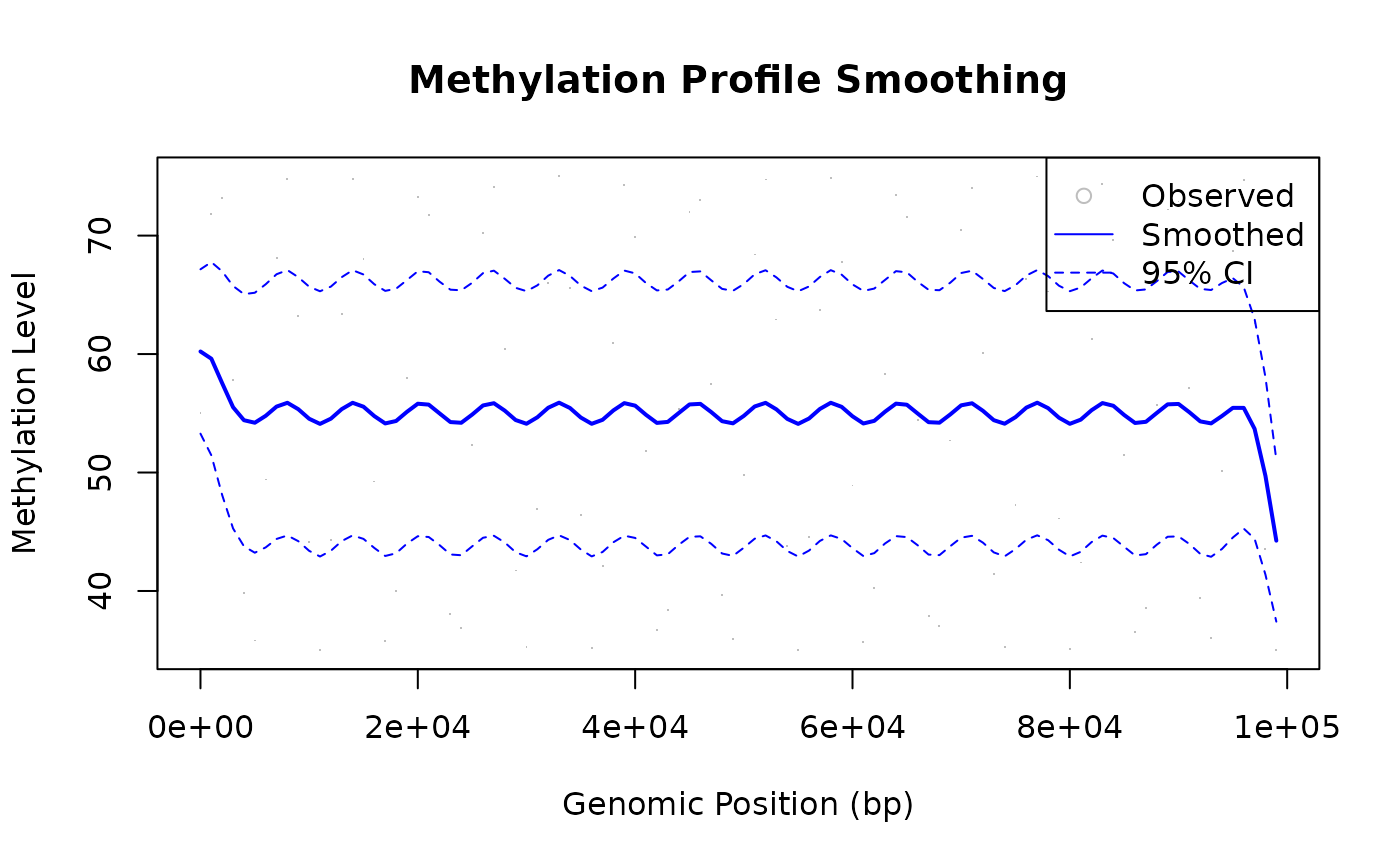

cat(sprintf(
    "95%% CI: [%.4f, %.4f]\n",
    result$confidence_lower[1], result$confidence_upper[1]
))
#> 95% CI: [53.2792, 67.1554]

---

ChIP-seq Signal Smoothing

Application

ChIP-seq experiments produce sparse, noisy coverage data. LOWESS can help identify binding regions.

fraction = 0.05 provides high spatial resolution — important for resolving narrow binding peaks that would otherwise be smeared into the background. The larger iterations = 5 is deliberate: Poisson-distributed read counts produce tall, isolated spikes, and extra robustness iterations progressively down-weight them so the estimated background level is not inflated by a handful of extreme counts.

library(rfastlowess)

positions <- seq(0, 99000, by = 1000)
signal <- 50 + sin(positions / 1000) * 20 + 5

model <- Lowess(
    fraction = 0.05,
    iterations = 5
)
result <- fit(model, positions, signal)

# Identify peaks above threshold
peak_count <- sum(result$y > 65.0)
cat(sprintf("y[0]: %.4f\n", result$y[1]))
#> y[0]: 59.9376
cat(sprintf("Peak count: %d\n", peak_count))
#> Peak count: 26

---

Large Genome Coverage (Streaming)

For whole-genome data that doesn’t fit in memory:

library(rfastlowess)

positions <- seq(0, 10000, by = 10)
coverage <- 50 + sin(positions / 100) * 20 + 5.0

model <- StreamingLowess(
    fraction = 0.05,
    iterations = 3,
    chunk_size = 50,
    overlap = 10,
    merge_strategy = "weighted_average"
)

process_chunk(model, positions, coverage)
#> <LowessResult>
#>   Points:            991 
#>   Fraction Used:     0.05 
#>   Iterations Used:   3
result <- finalize(model)
cat(sprintf("y[0]: %.4f\n", result$y[1]))
#> y[0]: 41.2839

---

Best Practices for Genomic Data

Consideration	Recommendation
Fraction	0.05–0.15 (preserve local features)
Iterations	3–5 (handle sequencing outliers)
Large data	Use streaming mode
Sparse regions	Use boundary_policy="extend"
Multiple chromosomes	Process separately or ensure sorted

---

See Also

• Concepts — How LOWESS works
• ?Lowess — All options
• Robustness — Outlier downweighting in depth
• Merge Strategies — Streaming chunk reconciliation
• Boundary Handling — Edge handling for sparse regions
• Real-Time Processing — For sequencing runs

sessionInfo()
#> R version 4.6.1 (2026-06-24)
#> Platform: x86_64-pc-linux-gnu
#> Running under: Ubuntu 24.04.5 LTS
#> 
#> Matrix products: default
#> BLAS:   /usr/lib/x86_64-linux-gnu/openblas-pthread/libblas.so.3 
#> LAPACK: /usr/lib/x86_64-linux-gnu/openblas-pthread/libopenblasp-r0.3.26.so;  LAPACK version 3.12.0
#> 
#> locale:
#>  [1] LC_CTYPE=C.UTF-8       LC_NUMERIC=C           LC_TIME=C.UTF-8       
#>  [4] LC_COLLATE=C.UTF-8     LC_MONETARY=C.UTF-8    LC_MESSAGES=C.UTF-8   
#>  [7] LC_PAPER=C.UTF-8       LC_NAME=C              LC_ADDRESS=C          
#> [10] LC_TELEPHONE=C         LC_MEASUREMENT=C.UTF-8 LC_IDENTIFICATION=C   
#> 
#> time zone: UTC
#> tzcode source: system (glibc)
#> 
#> attached base packages:
#> [1] stats     graphics  grDevices utils     datasets  methods   base     
#> 
#> other attached packages:
#> [1] rfastlowess_5.0.0
#> 
#> loaded via a namespace (and not attached):
#>  [1] digest_0.6.39     desc_1.4.3        R6_2.6.1          fastmap_1.2.0    
#>  [5] xfun_0.61         cachem_1.1.0      knitr_1.52        htmltools_0.5.9  
#>  [9] rmarkdown_2.32    lifecycle_1.0.5   cli_3.6.6         sass_0.4.10      
#> [13] pkgdown_2.2.1     textshaping_1.0.5 jquerylib_0.1.4   systemfonts_1.3.2
#> [17] compiler_4.6.1    tools_4.6.1       ragg_1.5.2        bslib_0.12.0     
#> [21] evaluate_1.0.5    yaml_2.3.12       otel_0.2.0        jsonlite_2.0.0   
#> [25] rlang_1.3.0       fs_2.1.0          htmlwidgets_1.6.4