Boundary Handling
Edge strategies that reduce bias near the ends of the data range.
Overview
Standard LOWESS neighbourhoods become asymmetric at the boundaries: fewer points exist on one side, pulling the local fit toward the data interior. The boundary_policy parameter controls how the data is padded to mitigate this effect.
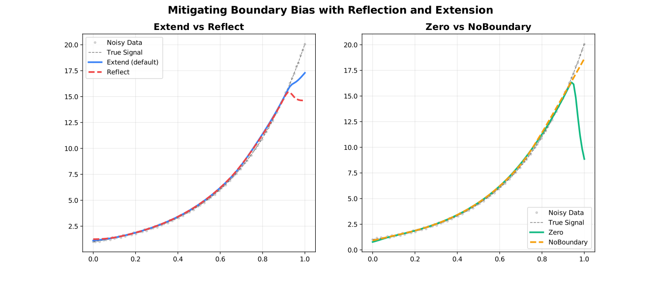
| Policy | Padding Strategy | Best For |
|---|---|---|
"extend" | Repeat first / last value | Most datasets (default) |
"reflect" | Mirror data at boundaries | Periodic or symmetric data |
"zero" | Pad with zeros | Data known to approach zero |
"noboundary" | No padding (Cleveland original) | Reproducing reference behaviour |
Extend (Default)
Pads beyond both endpoints by replicating the first and last observed values. Prevents the fit from curling toward zero and is a safe default for nearly all use cases.
Use when: No strong prior on boundary behaviour; general-purpose smoothing.
using FastLOWESS
using Random, Statistics

rng = MersenneTwister(42)
x = collect(range(0, 2π, length=100))
y = sin.(x) .+ randn(rng, 100) .* 0.3

model = Lowess(; boundary_policy="extend")
result = fit(model, x, y)
println("First smoothed value (extend policy): ", result.y[1])
First smoothed value (extend policy): 0.4426033958974517Reflect
Mirrors the data about both endpoints before fitting, then discards the reflected region from the output. Preserves continuity of derivatives, making it ideal for periodic or spatially symmetric signals.
Use when: Circular data (e.g., angle, day-of-year), symmetric physical quantities, or when the derivative at the boundary should be near zero.
using FastLOWESS
using Random, Statistics

rng = MersenneTwister(42)
x = collect(range(0, 2π, length=100))
y = sin.(x) .+ randn(rng, 100) .* 0.3

model = Lowess(; boundary_policy="reflect")
result = fit(model, x, y)
println("First smoothed value (reflect policy): ", result.y[1])
First smoothed value (reflect policy): 0.5294417978411072Zero
Pads with zeros beyond both endpoints. Appropriate when the underlying process is known to be zero outside the observation window (e.g., a pulse signal or a bounded physical quantity).
Use when: Signal decays to zero at both ends; zero is a meaningful boundary value.
using FastLOWESS
using Random, Statistics

rng = MersenneTwister(42)
x = collect(range(0, 2π, length=100))
y = sin.(x) .+ randn(rng, 100) .* 0.3

model = Lowess(; boundary_policy="zero")
result = fit(model, x, y)
println("First smoothed value (zero policy): ", result.y[1])
First smoothed value (zero policy): 0.26233331300426266No Boundary
Applies no padding. Each local fit uses only the points that are actually available, which may be fewer than the requested neighbourhood at the endpoints. This reproduces the original Cleveland (1979) algorithm exactly.
Use when: Reproducing reference results; you prefer the raw LOWESS boundary behaviour.
Without padding, boundary fits can have higher variance and visible edge artefacts, particularly with small fraction values.
using FastLOWESS
using Random, Statistics

rng = MersenneTwister(42)
x = collect(range(0, 2π, length=100))
y = sin.(x) .+ randn(rng, 100) .* 0.3

model = Lowess(; boundary_policy="noboundary")
result = fit(model, x, y)
println("First smoothed value (noboundary policy): ", result.y[1])
First smoothed value (noboundary policy): 0.5190958474065474Choosing a Policy
| Situation | Recommended Policy |
|---|---|
| General purpose | "extend" (default) |
| Periodic signal (angle, day-of-year) | "reflect" |
| Signal known to be zero at boundaries | "zero" |
| Replicating original Cleveland behaviour | "noboundary" |