Understanding how LOWESS works and when to use it.
What is LOWESS?#
LOWESS (Locally Weighted Scatterplot Smoothing) is a nonparametric regression method that fits smooth curves through scatter plots without assuming a global functional form.
Unlike parametric methods (linear regression, polynomial fitting), LOWESS adapts locally to the data structure, making it ideal for:
- Exploratory data analysis — Discover patterns without assumptions
- Trend estimation — Extract signals from noisy time series
- Baseline correction — Remove systematic effects in spectroscopy
- Genomic smoothing — Smooth methylation, ChIP-seq, or expression data
How It Works#
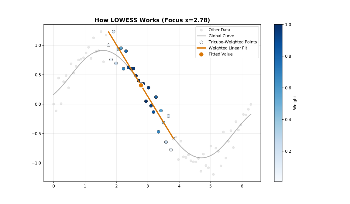
LOWESS fits local weighted regressions at each point, using a focused local window around each evaluation point
For each point in your data, LOWESS:
- Selects neighbors — Choose the nearest points (controlled by
fraction) - Assigns weights — Closer points get higher weights (using a kernel function)
- Fits locally — Perform weighted least squares regression
- Extracts value — Use the fitted value as the smoothed estimate
- Iterates (optional) — Reweight points based on residuals to reduce outlier influence
The Fraction Parameter#
fraction (also called bandwidth or span) is the most important parameter. It controls what proportion of data is used for each local fit.
| Fraction | Effect | When to Use |
|---|---|---|
| 0.1–0.3 | Fine detail, follows data closely | Rapidly changing signals |
| 0.3–0.5 | Balanced smoothing | Most applications |
| 0.5–0.7 | Heavy smoothing | Noisy data, trend extraction |
| 0.7–1.0 | Very smooth | Strong noise, global trends |
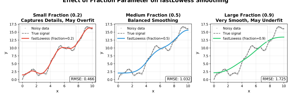
Small fraction vs large fraction — bandwidth controls how closely the fit follows local structure
Rule of Thumb: Start with
fraction = 0.67(the default) and adjust based on visual inspection. Use cross-validation for automated selection.
Robustness Iterations#
Standard LOWESS is sensitive to outliers. Robustness iterations downweight points with large residuals:
| Iterations | Effect | When to Use |
|---|---|---|
| 0 | No robustness (fastest) | Clean data, speed-critical |
| 1–3 | Moderate robustness | Most applications |
| 4–6 | Strong robustness | Data with outliers |
| 7+ | Very strong | Heavy contamination |
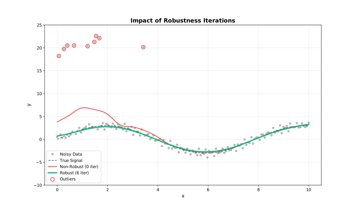
Non-robust LOWESS (iterations=0) vs robust LOWESS — outlier influence is suppressed through iterative reweighting
Confidence vs Prediction Intervals#
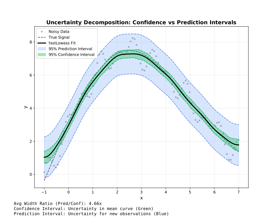
Confidence intervals (narrow, mean curve uncertainty) vs Prediction intervals (wide, new-point uncertainty)
| Interval Type | What It Represents | Width |
|---|---|---|
| Confidence | Uncertainty in the mean curve | Narrow |
| Prediction | Uncertainty for new observations | Wide |
- Use confidence intervals to show where the true trend likely lies
- Use prediction intervals to show where new data points might fall
Execution Modes#
Choose the right mode based on your use case:
| Mode | Use Case | Memory | Features |
|---|---|---|---|
Lowess (batch) | Complete datasets | Entire dataset | All features |
StreamingLowess | Large files (>100K points) | One chunk | Residuals, robustness |
OnlineLowess | Real-time data | Fixed window | Incremental updates |
Quick Decision Guide#
| Situation | Mode |
|---|---|
| Data fits in memory; needs intervals or CV | Lowess |
| Data too large for memory or arrives in chunks | StreamingLowess |
| Data arrives point-by-point in real time | OnlineLowess |
See Execution Modes for a fuller comparison.
Key Advantages#
| Feature | LOWESS | Polynomial Regression | Moving Average |
|---|---|---|---|
| No parametric assumptions | ✓ | ✗ | ✓ |
| Adapts to local structure | ✓ | ✗ | Partial |
| Robust to outliers | ✓ | ✗ | ✗ |
| Uncertainty estimates | ✓ | ✓ | ✗ |
| Handles irregular sampling | ✓ | ✓ | ✗ |
Next Steps#
- Getting Started — See it in action
- API Reference — All configuration options
- Boundary Handling — Edge bias reduction strategies
- Robustness — Outlier downweighting methods
- Scaling Methods — MAD, MAR, Mean scale estimation
- Merge Strategies — Chunk reconciliation in Streaming mode